Evaluation Metrics For Regression
Regression refers to predictive modeling problems that involve predicting a numeric value.

It is different from the classification that involves predicting a class label. Unlike classification, you cannot use classification accuracy to evaluate the predictions made by a regression model.
I have wrote article on evaluation metrics for classification task you can checkout here .
Instead, you must use error metrics specifically designed for evaluating predictions made on regression problems.
In this article, you will discover how to calculate error metrics for regression predictive modeling projects.
Regression Predictive Modeling:
Predictive modeling is the problem of developing a model using historical data to make a prediction on new data where we do not have the answer.
Predictive modeling can be described as the mathematical problem of approximating a mapping function (f) from input variables (X) to output variables (y). This is called the problem of function approximation.
The job of the modeling algorithm is to find the best mapping function we can given the time and resources available.
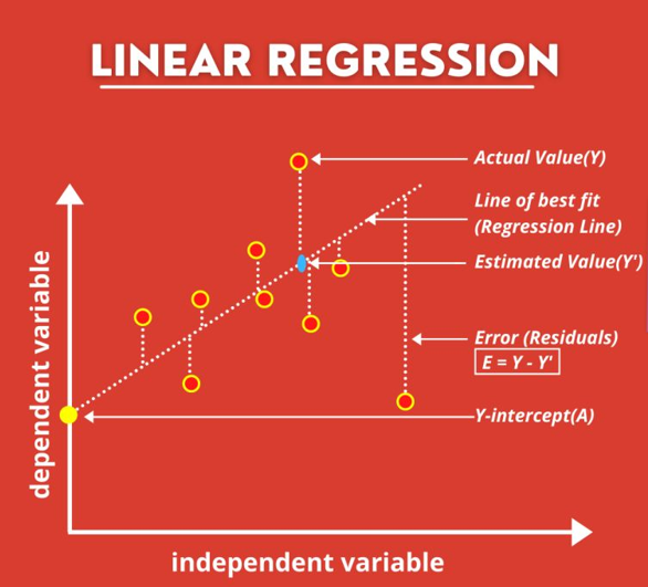
Regression predictive modeling is the task of approximating a mapping function (f) from input variables (X) to a continuous output variable (y).
Regression is different from classification, which involves predicting a category or class label.
- A regression problem requires the prediction of a quantity.
- A regression can have real-valued or discrete input variables.
- A problem with multiple input variables is often called a multivariate regression problem.
- A regression problem where input variables are ordered by time is called a time series forecasting problem.
Now that we are familiar with regression predictive modeling, let’s look at how we might evaluate a regression model.
Evaluating Regression Models:
There are three error metrics that are commonly used for evaluating and reporting the performance of a regression model; they are:
- Mean Squared Error (MSE).
- Root Mean Squared Error (RMSE).
- Mean Absolute Error (MAE)
There are many other metrics for regression, although these are the most commonly used.We will some other metrics as well.
You can see the full list of regression metrics supported by the scikit-learn Python machine learning library here:
Mean Squared Error:
The most common metric for regression tasks is MSE.
It is also an important loss function for algorithms fit or optimized using the least-squares framing of a regression problem. Here “least squares” refers to minimizing the mean squared error between predictions and expected values.
Loss Function Must have two properties :
- The function must be differentiable
- The function must be convex in nature
And MSE fulfills both the requirements to be loss function.

The squaring also has the effect of inflating or magnifying large errors. That is, the larger the difference between the predicted and expected values, the larger the resulting squared positive error. This has the effect of “punishing” models more for larger errors when MSE is used as a loss function. It also has the effect of “punishing” models by inflating the average error score when used as a metric.

The individual error terms are averaged so that we can report the performance of a model with regard to how much error the model makes generally when making predictions, rather than specifically for a given example.
The units of the MSE are squared units.
For example, if your target value represents “dollars,” then the MSE will be “squared dollars.” This can be confusing for stakeholders; therefore, when reporting results, often the root mean squared error is used instead (discussed in the next section).
The mean squared error between your expected and predicted values can be calculated using the mean_squared_error() function from the scikit-learn library.
Running the example calculates and prints the mean squared error get 0.35 sq. unit
A perfect mean squared error value is 0.0, which means that all predictions matched the expected values exactly.
It is a good idea to first establish a baseline MSE for your dataset using a naive predictive model, such as predicting the mean target value from the training dataset. A model that achieves an MSE better than the MSE for the naive model has skill.
Root Mean Squared Error
The Root Mean Squared Error, or RMSE, is an extension of the mean squared error.
Importantly, the square root of the error is calculated, which means that the units of the RMSE are the same as the original units of the target value that is being predicted.
For example, if your target variable has the units “dollars,” then the RMSE error score will also have the unit “dollars” and not “squared dollars” like the MSE.
As such, it may be common to use MSE loss to train a regression predictive model, and to use RMSE to evaluate and report its performance.
- The power of ‘square root’ empowers this metric to show large number deviations.
- The ‘squared’ nature of this metric helps to deliver more robust results which prevent canceling the positive and negative error values. In other words, this metric aptly displays the plausible magnitude of the error term.
- It avoids the use of absolute error values which is highly undesirable in mathematical calculations.
- When we have more samples, reconstructing the error distribution using RMSE is considered to be more reliable.
- RMSE is highly affected by outlier values. Hence, make sure you’ve removed outliers from your data set prior to using this metric.
- As compared to mean absolute error, RMSE gives higher weightage and punishes large errors.

where N is the Total Number of Observations.

We can see the plot is linear. This because RMSE = sqrt(MSE) will give linear error function.
Running the example calculates and prints the mean squared error get 0.5916 unit.
A perfect RMSE value is 0.0, which means that all predictions matched the expected values exactly.
Mean Absolute Error
Mean Absolute Error, or MAE is a popular metric because, like RMSE, the units of the error score match the units of the target value that is being predicted.
Unlike the RMSE, the changes in MAE are linear and therefore intuitive.
That is, MSE and RMSE punish larger errors more than smaller errors, inflating or magnifying the mean error score. This is due to the square of the error value. The MAE does not give more or less weight to different types of errors and instead the scores increase linearly with increases in error.
As its name suggests, the MAE score is calculated as the average of the absolute error values. Absolute or abs() is a mathematical function that simply makes a number positive. Therefore, the difference between an expected and predicted value may be positive or negative and is forced to be positive when calculating the MAE.

The example below gives a small contrived dataset of all 1.0 values and predictions that range from perfect (1.0) to wrong (0.0) by 0.1 increments. The absolute error between each prediction and expected value is calculated and plotted to show the linear increase in error.
A line plot is created showing the straight line or linear increase in the absolute error value as the difference between the expected and predicted value is increased.

The mean absolute error between your expected and predicted values can be calculated using the mean_absolute_error() function from the scikit-learn library.
Running the example calculates and prints the mean absolute error. we get 0.5 unit
A perfect mean absolute error value is 0.0, which means that all predictions matched the expected values exactly.
It is a good idea to first establish a baseline MAE for your dataset using a naive predictive model, such as predicting the mean target value from the training dataset. A model that achieves a MAE better than the MAE for the naive model has skill.
R Square/Adjusted R Square
R Square measures how much of variability in dependent variable can be explained by the model. It is square of Correlation Coefficient(R) and that is why it is called R Square.
First we will see some terminolgy,

In regression, Simplest model you can build is baseline model (Avg. Model). Where for every input data point (xi)model will predict mean(yi) as predicted output.

MSE(baseline): Mean Squared Error of mean prediction against the actual values
After training model, Model will predicts output for every data points then we calculate MSE which is called as square of sum of residue given as,

So, finally R-squared is given as,

Now we will see boundary conditions,

Best value for R squared is 1.
Adjusted R-Squared
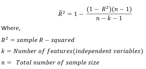
A model performing equal to baseline would give R-Squared as 0. Better the model, higher the R-Squared value. The best model with all correct predictions would give R-Squared as 1. However, on adding new features to the model, the R-Squared value either increases or remains the same. R-Squared does not penalize for adding features that add no value to the model. So an improved version over the R-Squared is the adjusted R-Squared. The formula for adjusted R-Squared is given by:

So, we can see Adujusted R-squared increases only when correlated independent features increases.
If R-Squared does not increase, that means the feature added isn’t valuable for our model. So overall we subtract a greater value from 1 and adjusted R-squared, in turn, would decrease.
Thus, the adjusted R-squared penalizes the model for adding furthermore independent variables (k in the equation) that do not fit the model.
Root Mean Squared Logarithmic Error
In case of Root mean squared logarithmic error, we take the log of the predictions and actual values. So basically, what changes are the variance that we are measuring. RMSLE is usually used when we don’t want to penalize huge differences in the predicted and the actual values when both predicted and true values are huge numbers.

- If both predicted and actual values are small: RMSE and RMSLE are same.
- If either predicted or the actual value is big: RMSE > RMSLE
- If both predicted and actual values are big: RMSE > RMSLE (RMSLE becomes almost negligible)
Conclusion
We discussed the most common evaluation metrics used in linear regression. We saw the metrics to use during multiple linear regression and model selection. Having gone over the use cases of most common evaluation metrics and selection strategies, I hope you understood the underlying meaning of the same.
Keep Learning, Happy Learning !!!
